Parsing Nested XML from Flying Probe Testers into a Relational Database

A Flying Probe Tester (FPT) is a PCB electrical validation machine. Instead of a custom bed-of-nails fixture, it uses motorized robotic probes that move across the board surface, touching test points and measuring resistance, capacitance, and continuity. For each board it tests, it generates an XML report — sometimes 5,000 nodes deep — describing every probe measurement, every pass/fail result, and every board-level metadata attribute.

Getting that XML into a queryable relational database is genuinely hard. The nesting is deep, the schemas drift between firmware versions, and the files are large enough that DOM parsing runs out of memory on edge hardware. Here's the architecture that handles it.

The Three-Table Schema

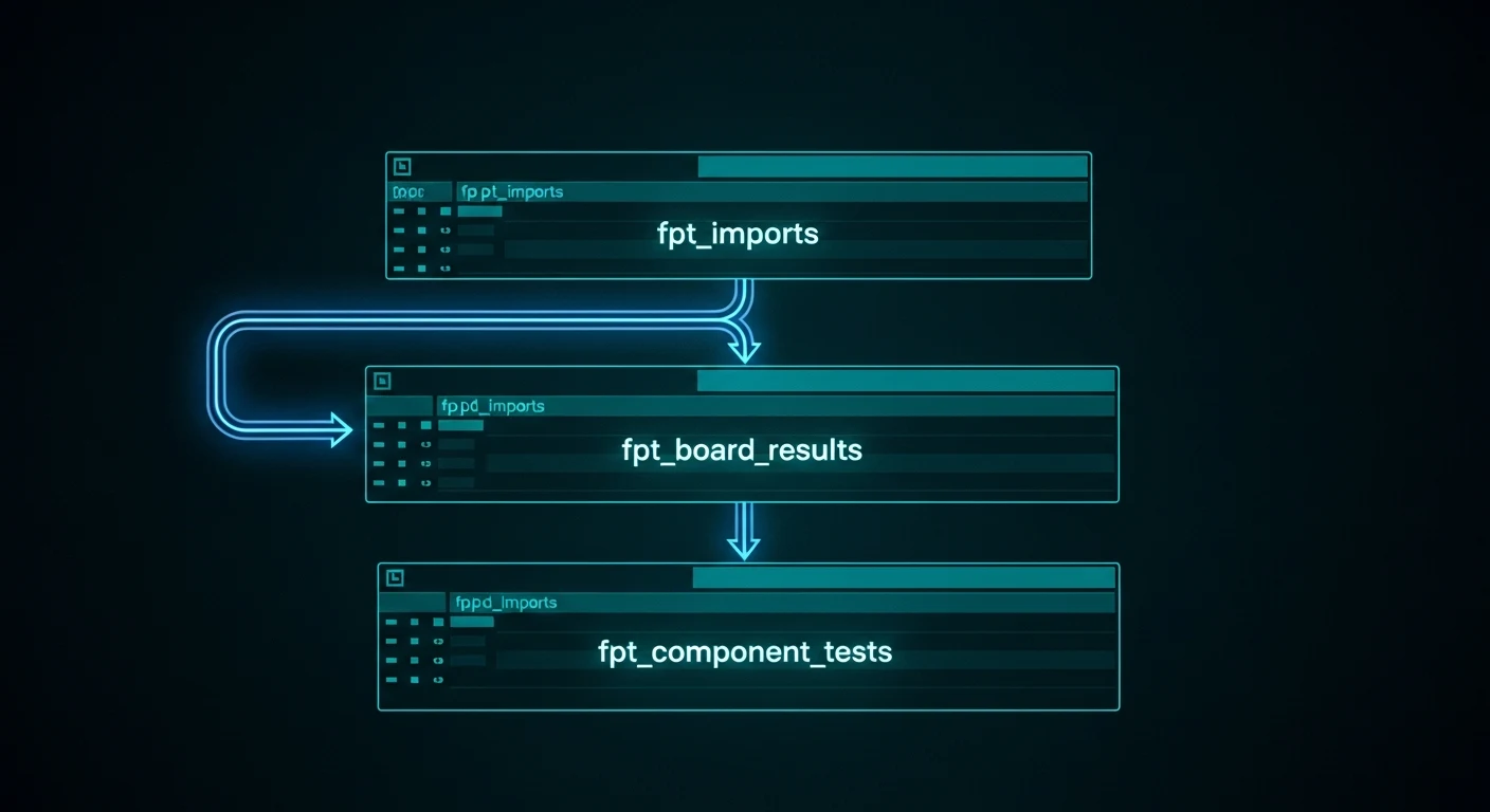
Hierarchical XML data maps naturally to a three-table relational schema with cascading foreign keys:

fpt_imports — One row per file import. Tracks the file path, import timestamp, operator, and overall pass/fail summary. This table is the anchor for everything downstream.

fpt_board_results — One row per board tested in the file. A single FPT run often tests multiple boards in a panel. This table holds board serial number, board-level pass/fail, test duration, and temperature at time of test. Foreign key to fpt_imports.

fpt_component_tests — One row per individual probe measurement. A single board generates hundreds to thousands of rows here — one for each component pin pair tested. This table holds component reference designator, pin identifiers, measured value, expected value, tolerance, and pass/fail status. Foreign key to fpt_board_results.

This structure enables queries at any level of granularity: "how many boards passed today?" hits fpt_board_results. "Which specific pin pairs are failing on resistor R47 across all boards this week?" hits fpt_component_tests with a join to fpt_board_results.

The Namespace Problem

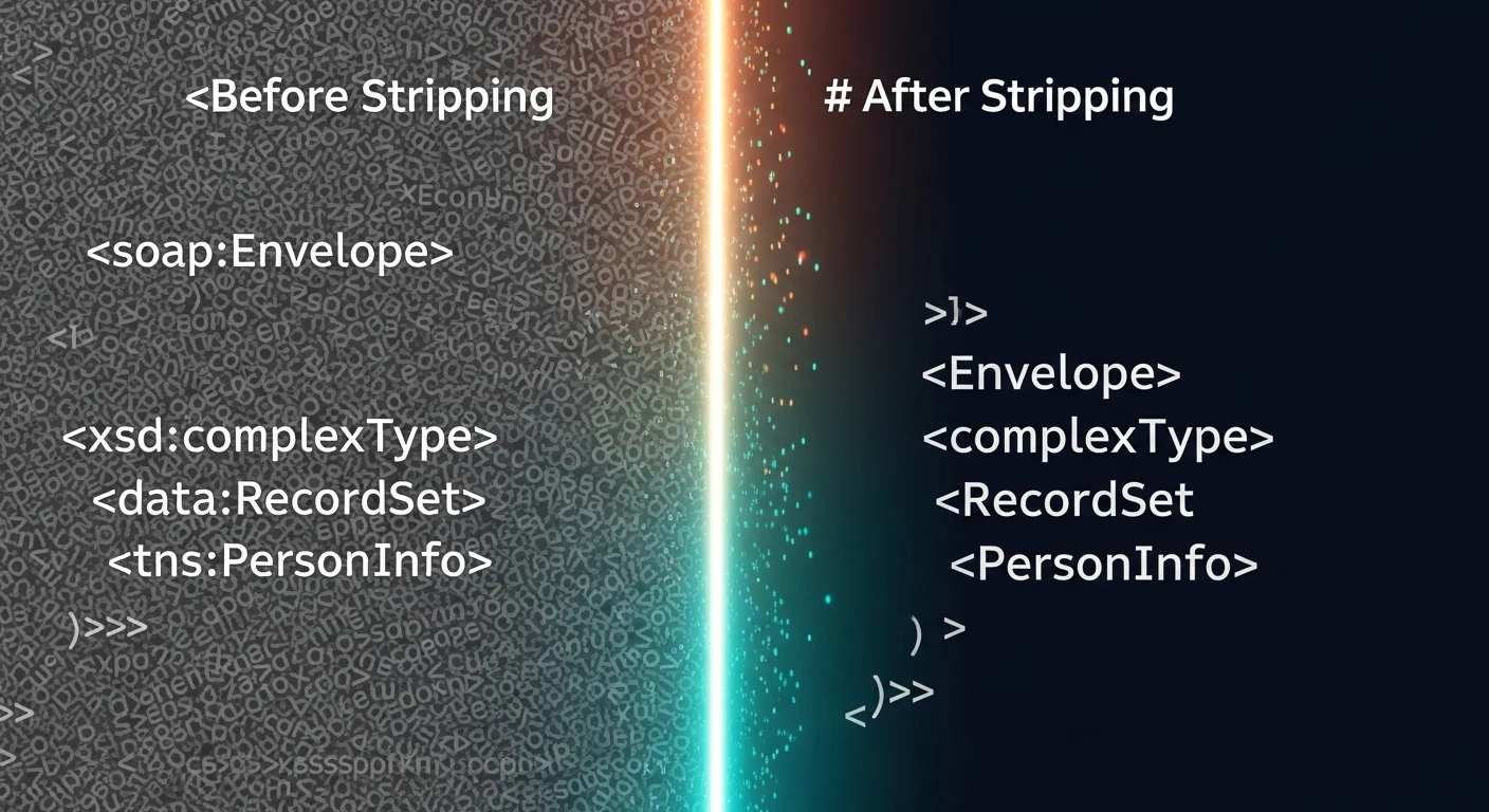
FPT XML files use XML namespaces — the xmlns declarations that look like xmlns:fpt="http://vendor.com/fpt/v2". In theory, namespaces make XML schemas extensible and version-stable. In practice, hardware vendors update firmware and silently change their namespace URIs, which breaks every namespace-aware parser that references the old URI.

The defensive solution is namespace-agnostic parsing using lxml's Clark notation normalization:

from lxml import etree
 
def strip_namespace(element):
    """Remove namespace prefix from tag name."""
    if '}' in element.tag:
        element.tag = element.tag.split('}', 1)[1]
    for child in element:
        strip_namespace(child)
    return element
 
def parse_fpt_file(filepath: str) -> etree._Element:
    tree = etree.parse(filepath)
    root = tree.getroot()
    return strip_namespace(root)

After stripping namespaces, XPath queries use bare tag names — ".//BoardResult" instead of ".//fpt:BoardResult". When the vendor updates their namespace URI in the next firmware release, the parser still works.

Streaming Parse for Large Files

FPT XML files for a full production shift can exceed 500MB. Loading the entire document into memory with etree.parse() works for small files; for large ones, it causes the Python process to exhaust available RAM on edge hardware.

The solution is iterative/streaming parsing using etree.iterparse(), which processes the XML document as a stream and yields elements as it encounters them. The key is the clear() call that discards processed elements from memory:

def stream_parse_component_tests(filepath: str):
    context = etree.iterparse(filepath, events=("end",), tag="ComponentTest")
    for event, elem in context:
        yield {
            "ref_des": elem.findtext("RefDes"),
            "pin_a": elem.findtext("PinA"),
            "pin_b": elem.findtext("PinB"),
            "measured": float(elem.findtext("Measured") or 0),
            "expected": float(elem.findtext("Expected") or 0),
            "passed": elem.findtext("Result") == "PASS"
        }
        elem.clear()  # ← critical: discard from memory after processing

Memory usage stays flat regardless of file size. A 500MB file processes in a constant ~40MB memory footprint.

Bulk Insert for Performance

With thousands of component test rows per board, inserting them one at a time with individual INSERT statements takes minutes. SQLite's executemany() with a transaction wrapping the entire batch reduces that to seconds:

def bulk_insert_component_tests(conn, board_id: int, tests: list[dict]):
    rows = [(board_id, t["ref_des"], t["pin_a"], t["pin_b"],
             t["measured"], t["expected"], t["passed"]) for t in tests]
    conn.executemany("""
        INSERT INTO fpt_component_tests 
        (board_id, ref_des, pin_a, pin_b, measured, expected, passed)
        VALUES (?, ?, ?, ?, ?, ?, ?)
    """, rows)
    conn.commit()

The transaction is critical — SQLite commits after each individual insert by default, which means thousands of disk syncs. Wrapping in a transaction means one disk sync for the entire batch.

Query Patterns That Emerge

Once the data is in the three-table schema, query patterns that were previously impossible become straightforward. Some examples that the assembly hub's analytics layer uses regularly:

Component failure rate by family: Join fpt_component_tests to the canonical component library on ref_des, group by family, and compute pass rate. Immediately surfaces whether capacitors or resistors are driving failures this week.

Board-to-board variation for the same part: Query all fpt_component_tests rows for a specific ref_des across all boards in a date range, and plot the distribution of measured values. A tight distribution indicates stable placement; a wide distribution indicates a machine or material problem.

Marginal pass analysis: Filter for rows where passed = TRUE but ABS(measured - expected) / expected > 0.8. These are components that passed this test but are operating near their tolerance limit — early warning of future failures.

The FPT data pipeline is genuinely complex to build but produces data that pays for itself every time an engineer uses it to diagnose a production issue before it becomes a field return.